How to Use IMPORTRANGE in Google Sheets? (2025 Guide)

Have you ever needed to pull data from one Google Sheet into another but didn’t want to manually copy and paste everything? That’s where IMPORTRANGE comes in. It’s a simple but powerful function that lets you automatically import data from one sheet to another, even if the sheets are in different files. Whether you’re consolidating information, tracking projects across multiple sheets, or just want to save time by keeping your data synced up, IMPORTRANGE makes it all possible with just a few clicks.

In this guide, we’ll walk through everything you need to know about using this handy tool, from the basics to advanced tips, so you can start making your Google Sheets work smarter and more efficiently.

What is IMPORTRANGE in Google Sheets?

The IMPORTRANGE function in Google Sheets is a powerful tool that allows you to import data from one spreadsheet into another. It makes it possible to pull information from a wide range of sources, even if those sources are in different files, and display it all in one location. This is especially useful when working with large sets of data or collaborating with others on multiple projects.

IMPORTRANGE is particularly helpful for users who need to manage data across various sheets and centralize that information without having to manually copy and paste data between documents. It automates the process of importing data and ensures that your destination sheet always reflects the latest updates from the source sheet.

Google Sheets IMPORTRANGE Function Syntax

IMPORTRANGE works by referencing a specific range in a source spreadsheet and bringing that data into a destination sheet. The formula for IMPORTRANGE consists of two main components:

1. Spreadsheet URL (or key) – This is the link or unique identifier for the source spreadsheet from which you want to pull data.
2. Range String – This refers to the exact range of cells in the source sheet that you want to import. It typically includes the sheet name and the cell range, such as "Sheet1!A1:B10".

By combining these components, IMPORTRANGE allows you to pull data from other sheets with just a few lines of code.

Importance of IMPORTRANGE in Google Sheets

IMPORTRANGE serves several important purposes for Google Sheets users:

• Efficient Data Management: It allows you to manage data from multiple sheets without needing to manually copy or update information. This saves time and reduces the risk of errors.
• Streamlined Collaboration: By allowing different users to contribute to separate sheets, IMPORTRANGE enables better collaboration without having to merge or manually share data.
• Dynamic Data Updates: Since IMPORTRANGE automatically updates the destination sheet whenever the source sheet is modified, you don’t have to worry about keeping everything synchronized.
• Data Consolidation: You can easily consolidate data from various sources into one sheet, making it easier to analyze and report on large datasets.
• Cross-Sheet Connections: IMPORTRANGE helps connect multiple Google Sheets across different files, enabling you to work with data spread out over several documents without having to duplicate it.

How IMPORTRANGE Connects Multiple Google Sheets

IMPORTRANGE works by allowing you to link multiple Google Sheets together. Each sheet remains independent, but IMPORTRANGE acts as a bridge, pulling data from one sheet and displaying it in another. This connection allows data to flow dynamically across various files, ensuring that each sheet can be updated and referenced in real-time.

For example, if you have a sales report in one spreadsheet and a team performance tracker in another, you can use IMPORTRANGE to pull specific sales data into the performance tracker. When the sales data is updated, the performance tracker will reflect those changes automatically. This connection between sheets eliminates the need for manual updates and allows you to work more efficiently across multiple projects.

Key Benefits of Google Sheets IMPORTRANGE

IMPORTRANGE offers several key benefits that make it a must-have function for Google Sheets users:

• Reduces Manual Data Entry: By automating data imports, IMPORTRANGE saves you from having to manually copy and paste data, which can be time-consuming and prone to errors.
• Enables Real-Time Data Updates: Once linked, the data in the destination sheet updates automatically whenever changes are made in the source sheet, ensuring that your information is always up to date.
• Improves Collaboration: With IMPORTRANGE, multiple users can work on different sheets, and data can be imported into a central sheet for easy access and analysis.
• Increases Efficiency: By consolidating data from multiple sources into one location, you can quickly analyze large datasets without having to navigate between multiple sheets.
• Customizable Data Import: You can specify exactly which data you want to import, whether it’s specific ranges or entire columns, giving you control over the data that’s pulled into your destination sheet.

Common Use Cases for IMPORTRANGE

IMPORTRANGE can be used in a wide variety of scenarios where pulling data from one sheet into another is necessary. Some common use cases include:

• Consolidating Data from Multiple Sheets: Pulling data from different sheets into one central sheet for easier analysis and reporting.
• Tracking Performance Metrics Across Teams: Aggregating data from individual team members’ sheets into one overall team performance tracker.
• Financial Reporting: Importing budget data from multiple departments into one spreadsheet to generate a comprehensive financial report.
• Project Management: Bringing data from multiple project trackers into one summary sheet to keep all team members aligned.
• Sales and Inventory Management: Importing sales and inventory data from separate product sheets to create a unified report for tracking business performance.

The Google Sheets IMPORTRANGE Function Syntax

Understanding the syntax of the IMPORTRANGE function is key to effectively using it to import data between Google Sheets. At its core, IMPORTRANGE requires two main elements: the URL of the source spreadsheet and the range of cells you want to pull data from. Let’s break down how each part works and how to use it in your own sheets.

The IMPORTRANGE Formula in Google Sheets

The basic syntax of the IMPORTRANGE formula is simple, but each part plays a crucial role in specifying what data is being pulled and from where. Here’s a closer look at each component of the formula:

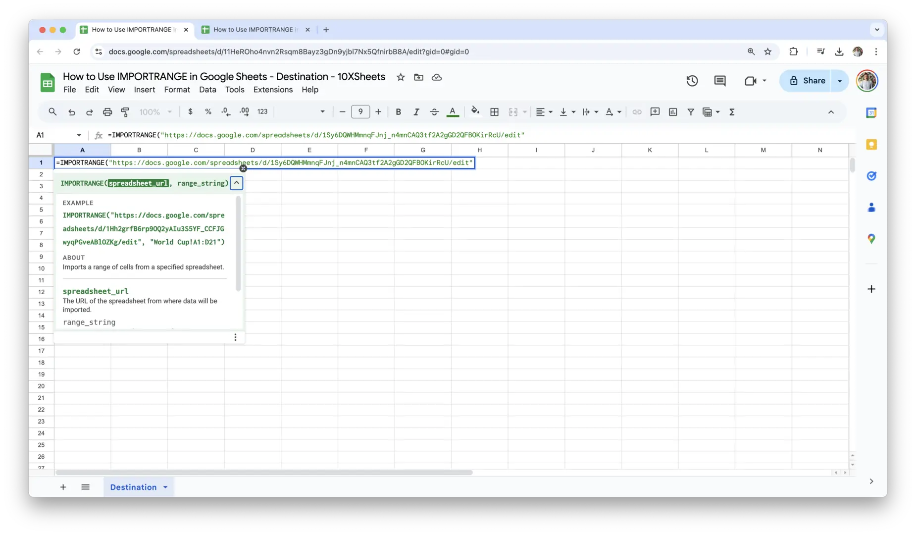
1. Spreadsheet URL: The first part of the formula is the URL of the spreadsheet from which you want to import data. This is the link to the source Google Sheet, and you can find it in the address bar when you have the sheet open. It’s important to enclose the URL in double quotation marks.
   • Example: "https://docs.google.com/spreadsheets/d/1abc123xyz456/edit"

   You can also use just the spreadsheet key (the part of the URL that’s unique to the sheet) instead of the full URL, but using the full URL makes it clearer what sheet you’re referencing.
   

2. Range String: The second part of the formula is the range of cells you want to import. This includes both the sheet name and the specific range of cells. The range string is written in this format: "SheetName!CellRange". The sheet name is followed by an exclamation mark, and then the range of cells, which can be anything from a single cell to an entire set of rows and columns.
   • Example: "Sheet1!A1:B10" pulls data from columns A and B, rows 1 through 10, from a sheet named “Sheet1”.

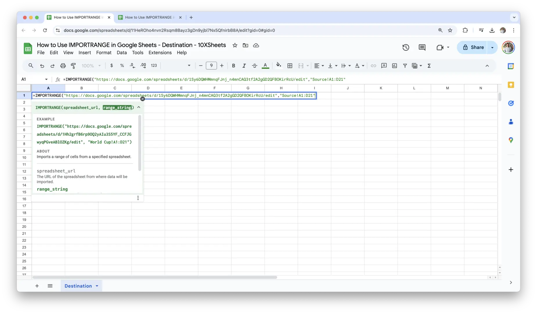
When combined, the formula takes the following form:

IMPORTRANGE("spreadsheet_url", "range_string")

It tells Google Sheets to fetch the data from the specified range in the source sheet and display it in the cell where the formula is used.

How to Write a Basic IMPORTRANGE Formula?

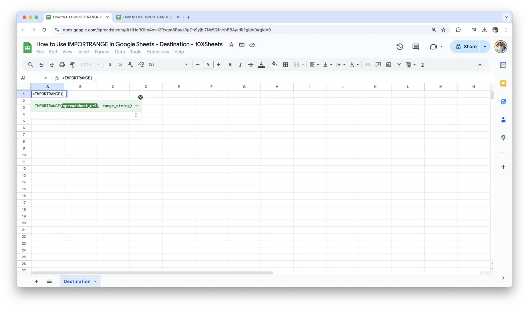
Writing a basic IMPORTRANGE formula follows a simple, step-by-step process. Let’s go through the procedure of creating and using the formula.

1. Get the URL of the Source Spreadsheet: To begin, open the Google Sheet from which you want to import data. Copy the full URL from the address bar of your browser. It should look something like this:

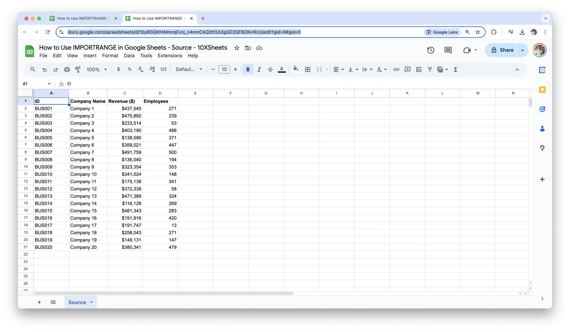
   https://docs.google.com/spreadsheets/d/1abc123xyz456/edit
   

2. Identify the Range to Import: Next, identify the specific range of cells you need from the source sheet. For example, if you want to import data from columns A to D, rows 1 to 21, you would reference "Source!A1:D21". Make sure you include the exact sheet name and the range of cells you want to pull.
3. Write the IMPORTRANGE Formula: Now, combine the spreadsheet URL and the range into the formula. Based on the examples above, the formula would look like this:

   =IMPORTRANGE("https://docs.google.com/spreadsheets/d/1abc123xyz456/edit", "Source!A1:D21")
   

   This formula tells Google Sheets to import data from the range A1:B10 on Sheet1 of the specified spreadsheet.

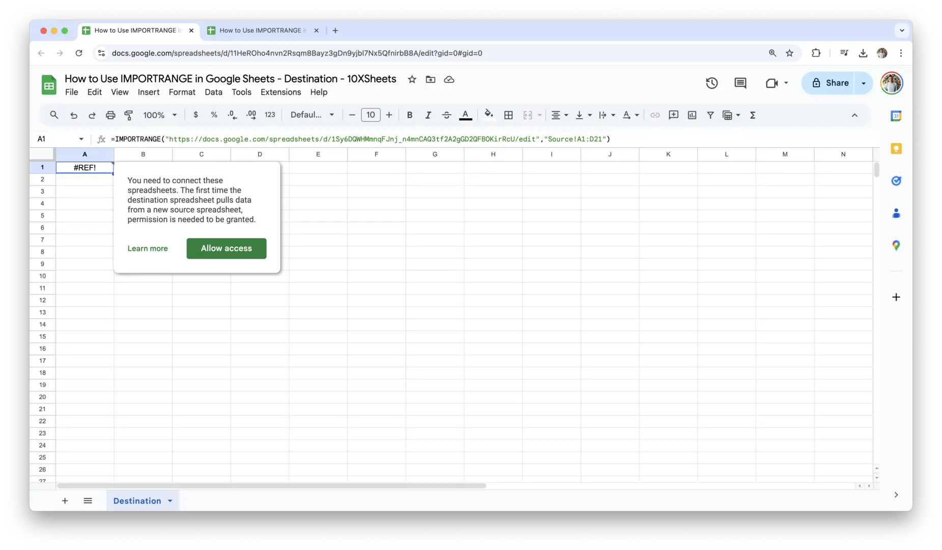
4. Allow Access: The first time you use IMPORTRANGE with a new sheet, Google Sheets will ask for permission to access the source spreadsheet. Once you click “Allow Access,” the data from the source sheet will be imported into your destination sheet.
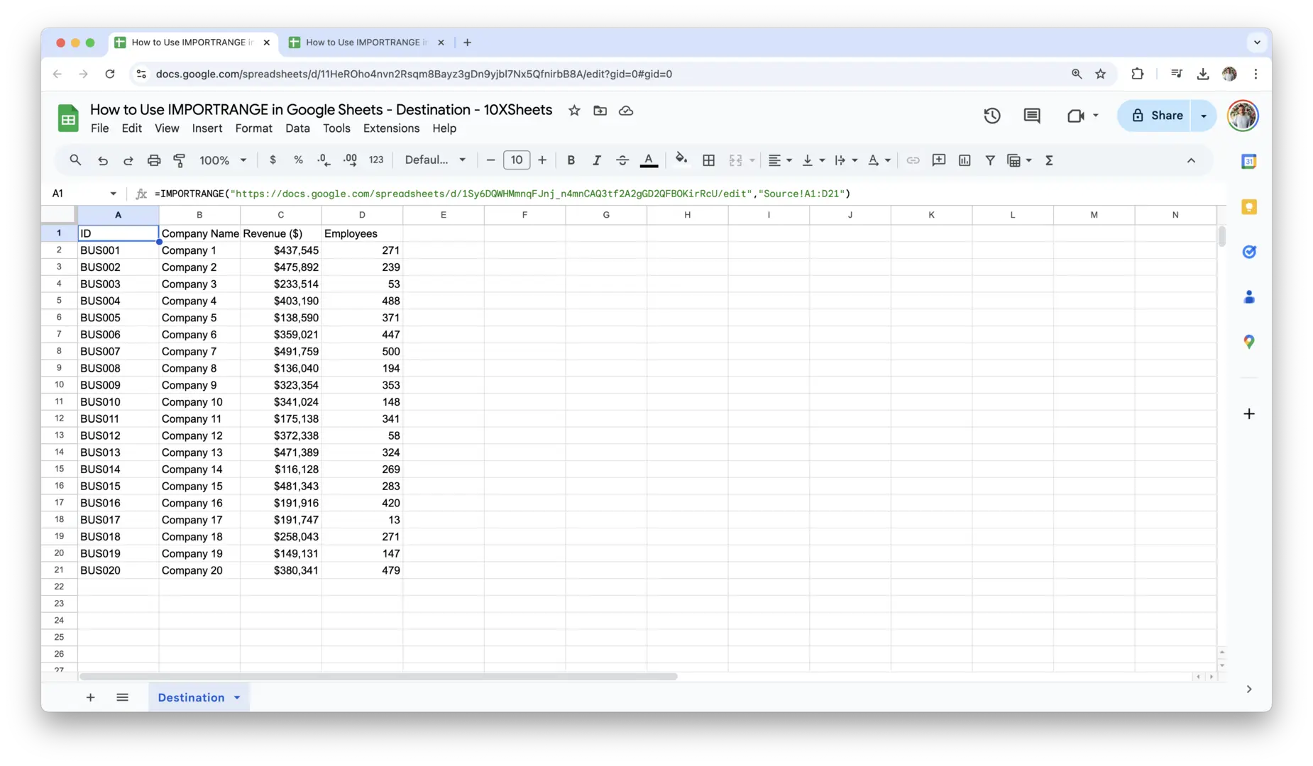
5. View the Imported Data: After granting permission, the data from the source sheet will automatically appear in your destination sheet at the location where you entered the formula. This data will stay updated, reflecting any changes made in the source sheet.

By following these simple steps, you can start using IMPORTRANGE to import data from one Google Sheet into another quickly and efficiently. This basic formula allows you to connect different sheets and centralize your information for easier analysis and reporting.

How to Use IMPORTRANGE in Google Sheets?

Using the IMPORTRANGE function is straightforward, but understanding the steps and knowing how to troubleshoot common issues can make the process even easier. Let’s break down the process of using IMPORTRANGE, from writing the formula to solving potential errors that may arise.

How to Use Google Sheets IMPORTRANGE?

The process of using IMPORTRANGE is fairly simple, but each step is essential to ensure that data is pulled correctly from one sheet to another. Here’s how to do it:

1. Open the Destination Sheet: First, open the Google Sheet where you want to display the imported data. This is where you’ll enter the IMPORTRANGE formula.
   
2. Find the Source Sheet URL: Go to the source Google Sheet—the one from which you want to pull the data. Open that sheet, and copy the URL from your browser’s address bar. You’ll need this URL to reference the source sheet in your formula.
   
3. Identify the Range You Want to Import: In the source sheet, identify the range of cells you want to pull into your destination sheet. This could be anything from a small range (e.g., A1:B10) to an entire column (e.g., A:A) or even an entire sheet (e.g., “Sheet1!A:Z”).
4. Write the IMPORTRANGE Formula: Go back to your destination sheet, and in the cell where you want the imported data to appear, type the IMPORTRANGE formula. For example, if the source sheet’s URL is:

   https://docs.google.com/spreadsheets/d/1abc123xyz456/edit
   

   And the range you want to import is Source!A2:D21, your formula will look like this:

   =IMPORTRANGE("https://docs.google.com/spreadsheets/d/1abc123xyz456/edit", "Source!A2:D21")
    

5. Grant Permission: The first time you use IMPORTRANGE to pull data from a specific sheet, Google Sheets will ask for permission to access the source sheet. Click Allow Access to enable the connection. Once permission is granted, the data from the source sheet will appear in your destination sheet.
   
6. Check the Data: The data should automatically fill in the destination sheet, updating dynamically whenever the source sheet is modified. You can now manipulate the data as needed using other functions or formulas.
   

By following these steps, you can easily pull data from one Google Sheet into another. It’s a quick way to centralize information and keep everything updated in real-time.

Practical Example of Pulling Data from Another Sheet

Let’s imagine you’re managing a project with multiple team members, each updating their own Google Sheets. You need to consolidate their data into one central sheet for analysis. Here’s how you would use IMPORTRANGE in this scenario:

1. Source Sheet: Each team member keeps their own task list in a separate Google Sheet. For instance, “Team A’s Task List” is located at the following URL:

   https://docs.google.com/spreadsheets/d/1abc123xyz456/edit
   

2. Range to Import: You need to import the task names and statuses from columns A and B (rows 1 to 20) of “Team A’s Task List.”
3. Formula in Destination Sheet: In your central Google Sheet, where you want all the team data to appear, enter the following IMPORTRANGE formula:

   =IMPORTRANGE("https://docs.google.com/spreadsheets/d/1abc123xyz456/edit", "Sheet1!A1:B20")
   

4. Result: Once permission is granted, the task names and statuses from “Team A’s Task List” will appear in your central sheet. You can repeat this process for other teams, and all the data will update automatically in your central sheet whenever someone updates their individual task list.

By using IMPORTRANGE in this way, you can easily aggregate data from multiple sources and keep everything synchronized without having to manually copy and paste information between sheets.

Common IMPORTRANGE Errors and How to Troubleshoot Them

While IMPORTRANGE is a powerful tool, there are a few common errors that users may encounter. Let’s go through some of them and how to resolve them.

1. #REF! Error: This is the most common error when using IMPORTRANGE. It usually appears when the source sheet hasn’t been granted access yet, or there’s an issue with the URL or range reference.
   How to Fix: If you see a #REF! error, make sure you’ve clicked Allow Access when prompted. Also, double-check that the URL is correct and that the range you’re trying to reference exists in the source sheet.
2. Permission Issues: If the source sheet is restricted and not shared with you, IMPORTRANGE won’t be able to pull data. This can happen if the source sheet is set to private or if you’re trying to access a sheet from another Google account.
   How to Fix: Ensure that the source sheet is shared with the Google account you’re using for the destination sheet. If you don’t have access, ask the sheet owner to share the document with you.
3. Broken Links: If the source sheet URL changes or if the source sheet is deleted, the IMPORTRANGE function will break, and the data will no longer be pulled.
   How to Fix: If the URL changes, you’ll need to update the IMPORTRANGE formula with the new URL. Similarly, if the source sheet is deleted, you’ll need to find a new source sheet and update your formula.
4. Incorrect Range Reference: If the range you’re referencing doesn’t exist (for example, trying to pull from a cell that is outside the data range), you’ll get an error or blank cells.
   How to Fix: Double-check the range string. Ensure that you’re referencing the correct sheet name and the correct range of cells. If you’re unsure, try referencing a smaller range to see if it pulls data correctly.
5. Formula Not Updating: Sometimes, the data might not update immediately after changes are made in the source sheet.
   How to Fix: Try refreshing both the source and destination sheets. You can also try editing the formula or making a small change to trigger the update.

By keeping these troubleshooting tips in mind, you can quickly resolve common issues and ensure that your IMPORTRANGE functions work as expected. This will help you avoid interruptions and ensure your data is always up-to-date and accurate.

Alternatives to IMPORTRANGE in Google Sheets

While IMPORTRANGE is an incredibly useful tool, there are times when you may want to explore other options for importing or managing data between Google Sheets. Here are some notable alternatives to consider:

• Google Apps Script: For more complex automation, Google Apps Script can be used to write custom scripts that pull data between sheets or even from external sources. It offers greater flexibility and control over the data import process.
• Google Sheets Add-ons: Add-ons like Supermetrics, Coupler.io, or Data Connector for Google Sheets can help automate data imports between multiple sources, including Google Sheets, CRMs, social media platforms, and databases.
• API Integrations: If you need to pull data from external systems or APIs, using Google Sheets’ built-in API connectors or third-party services like Make or Zapier can automate data import from a wide variety of sources.
• Linked Sheets: Google Sheets now allows you to link sheets from other files directly into one document. This method can sometimes offer a more seamless integration if you’re working with other Google products like Google Docs or Google Slides.
• Manual Imports: For smaller datasets or one-time imports, you can download CSV files from other spreadsheets or systems and upload them manually into your Google Sheets.

Each of these alternatives provides varying levels of customization and complexity, so it’s important to choose the one that best fits your needs based on the scale of your project and the type of data you’re handling.

Advanced Google Sheets IMPORTRANGE Features

IMPORTRANGE is a versatile function, and when combined with other functions like FILTER and QUERY, it becomes even more powerful. Let’s explore how you can enhance your use of IMPORTRANGE to tackle more complex data needs and work with larger datasets more efficiently.

Using IMPORTRANGE with Other Functions Like FILTER and QUERY

While IMPORTRANGE allows you to import data, combining it with other functions like FILTER and QUERY gives you the ability to refine and manipulate that data before it’s displayed in your destination sheet. This can be especially useful when you want to apply conditions or perform specific calculations on the imported data.

Example: Using IMPORTRANGE with FILTER

Let’s say you have a source sheet that contains sales data for various products, and you want to pull only the rows where the sales amount is greater than $1,000. Instead of importing all the data and manually filtering it, you can combine IMPORTRANGE with the FILTER function to automatically pull just the rows you need.

Here’s how the formula would look:

=FILTER(IMPORTRANGE("https://docs.google.com/spreadsheets/d/1abc123xyz456/edit", "Sales!A2:C100"), IMPORTRANGE("https://docs.google.com/spreadsheets/d/1abc123xyz456/edit", "Sales!C2:C100") > 1000)

In this example:

• IMPORTRANGE imports the sales data from the source sheet.
• FILTER then ensures that only rows where the sales amount (in column C) is greater than 1000 are displayed.

This makes it easy to pull relevant data without needing to manually sort or filter after importing.

Example: Using IMPORTRANGE with QUERY

Another advanced function to pair with IMPORTRANGE is QUERY, which allows you to perform more complex operations on the imported data, like sorting, aggregating, or filtering with SQL-like syntax.

Suppose you want to pull sales data from the source sheet but only include rows where the sales amount exceeds $500 and sort the results by product name. You could combine IMPORTRANGE with QUERY like this:

=QUERY(IMPORTRANGE("https://docs.google.com/spreadsheets/d/1abc123xyz456/edit", "Sales!A2:C100"), "SELECT Col1, Col2, Col3 WHERE Col3 > 500 ORDER BY Col2", 1)

In this formula:

• IMPORTRANGE imports the sales data.
• QUERY filters out rows where the sales amount in column C is below $500 and orders the results by product name in column B.

By using QUERY with IMPORTRANGE, you can customize how the data is pulled and displayed in the destination sheet, making it more dynamic and suited to your needs.

Combining Multiple IMPORTRANGE Formulas for Dynamic Reports

IMPORTRANGE doesn’t have to be used in isolation. You can combine multiple IMPORTRANGE formulas to create more complex reports, especially if you’re pulling data from multiple sources or working with various ranges within a single source sheet.

Let’s say you’re compiling data for a report that requires sales figures from different sheets. Instead of importing data from each sheet separately and combining them manually, you can use ARRAYFORMULA or functions like VLOOKUP to automatically pull in data from multiple IMPORTRANGE formulas.

Example with ARRAYFORMULA:

=ARRAYFORMULA({IMPORTRANGE("https://docs.google.com/spreadsheets/d/1abc123xyz456/edit", "Sales Q1!A2:B10"); IMPORTRANGE("https://docs.google.com/spreadsheets/d/1abc123xyz456/edit", "Sales Q2!A2:B10")})

In this case, the formula combines two IMPORTRANGE formulas—one for Q1 data and one for Q2—into a single report. The ARRAYFORMULA function allows you to concatenate these two ranges vertically, creating a dynamic report with data from both sheets. This is extremely helpful for reports that aggregate data over multiple periods, regions, or projects.

Handling Large Datasets Efficiently

When working with large datasets, efficiency becomes a critical factor. IMPORTRANGE pulls data in real-time, which means that the more data you import, the longer it may take for your sheet to load or update. To handle large datasets efficiently, here are a few strategies:

• Limit Data Import: Instead of pulling an entire sheet, try to limit the data range to only what you need. For example, if you only need data from the last 100 rows, reference just that range ("Sheet1!A1:B100").
• Use Specific Queries: If you only need certain rows or columns, use QUERY or FILTER functions to pull only the data that meets your criteria, rather than importing an entire dataset.
• Split Large Imports: If you have an enormous dataset, consider splitting it into smaller chunks. Instead of using one huge IMPORTRANGE formula that pulls everything at once, break it into several smaller formulas for better performance.

By understanding how to combine IMPORTRANGE with other functions and working smartly with large datasets, you can create more efficient and dynamic reports without slowing down your Google Sheets.

IMPORTRANGE Use Cases

IMPORTRANGE is incredibly flexible, and its applications extend across many use cases, especially when working with multiple sheets and large datasets. Let’s explore a few practical scenarios where IMPORTRANGE can be especially useful.

Collaborative Team Projects and Shared Data

When managing team projects, it’s common for team members to work in separate Google Sheets, each maintaining their own individual data. With IMPORTRANGE, you can easily pull information from various sources into one central sheet. This eliminates the need to duplicate data and ensures everyone is working with the most up-to-date information.

For example, imagine you’re overseeing a marketing campaign, and each team member is tracking their own KPIs in separate sheets. Rather than manually collecting data or waiting for others to send it to you, you can set up IMPORTRANGE formulas in your central sheet to automatically pull in each person’s data. This makes collaboration smoother and reduces the risk of errors caused by outdated information.

Data Consolidation for Reporting Purposes

IMPORTRANGE is ideal for consolidating data from various sources into one master sheet. If you’re preparing a report that includes data from multiple teams, departments, or even external partners, IMPORTRANGE allows you to automate the process of collecting data into one location.

For instance, you could have multiple sheets that track sales by region, and you want to consolidate them into a single global sales report. Using IMPORTRANGE, you can pull in the data from each regional sheet and combine them into one report, all while keeping it dynamically updated. This is particularly useful when dealing with monthly or quarterly reports that need to aggregate data from multiple contributors.

Managing Large Databases Across Multiple Sheets

IMPORTRANGE can also be used to manage large databases that are spread across multiple sheets. Whether you’re organizing inventory, customer information, or project timelines, IMPORTRANGE helps keep everything in sync and reduces the need to manually update multiple sheets.

For example, in a product database, you may have information like product details, stock levels, and sales data in different sheets. By using IMPORTRANGE, you can create a central sheet that pulls all the necessary data into one location. This is not only efficient but also ensures that all sheets are consistently updated, making it easier to track and manage large datasets across your organization.

Whether you’re collaborating on a team project, consolidating data for a report, or managing an extensive database, IMPORTRANGE makes it easier to work with multiple sheets and keep everything in sync, saving you time and effort.

Troubleshooting IMPORTRANGE in Google Sheets

Although IMPORTRANGE is generally reliable, you may encounter some issues when working with it. These common problems can be resolved with a few simple steps:

• #REF! Error: This is often due to permission issues. Ensure that you have granted access to the source sheet and that the range you’re referring to is correct.
• Broken Link to Source Sheet: If the source sheet is deleted, renamed, or moved, IMPORTRANGE will no longer work. Double-check that the URL is correct and that the source sheet still exists.
• Permission Denied: If the source sheet is not shared with you, you’ll encounter a permission error. Make sure the sheet is shared with the appropriate Google account and that the necessary permissions are in place.
• Slow Performance: If you’re importing a large dataset or using multiple IMPORTRANGE functions in one sheet, it can cause slow load times. Consider breaking down large data imports into smaller ranges or using alternatives like QUERY to filter data before importing.
• Data Not Updating: Sometimes the data may not refresh automatically. Refresh both the source and destination sheets or re-enter the formula to trigger an update.
• Incorrect Range: Ensure the range you are referencing exists in the source sheet. If you’re unsure, test with a smaller range or check the source sheet to confirm the correct cell references.

By keeping these troubleshooting steps in mind, you’ll be able to quickly resolve issues and get your IMPORTRANGE formulas back on track.

Google Sheets IMPORTRANGE Best Practices

To get the most out of IMPORTRANGE and ensure smooth performance when working with multiple Google Sheets, here are some best practices to follow:

• Limit Data to What’s Necessary: Only import the data you need rather than pulling entire sheets. This keeps your destination sheet manageable and helps with performance.
• Use Specific Range References: Always specify the exact range you want to pull from the source sheet to avoid importing unnecessary data.
• Regularly Update Permissions: Make sure that the necessary permissions are always in place for the source sheets. If the source sheet owner changes settings or access, IMPORTRANGE may stop working.
• Keep Sheet Names Consistent: Use clear, logical naming conventions for your sheets to make it easier to reference them in IMPORTRANGE formulas.
• Avoid Overloading with Multiple IMPORTRANGE Functions: If you need to pull data from multiple sheets, try combining multiple ranges into one formula using functions like ARRAYFORMULA to avoid cluttering your destination sheet with too many individual IMPORTRANGE formulas.
• Use QUERY or FILTER for Data Manipulation: Instead of importing large datasets and manually cleaning them up, combine IMPORTRANGE with QUERY or FILTER functions to import only the relevant rows or columns you need.
• Monitor Performance: If your sheet starts to slow down, consider splitting large imports into smaller ranges or removing unnecessary formulas to improve load times.
• Test Small Ranges First: When setting up a new IMPORTRANGE formula, test it with a small range of data first to ensure the formula works as expected before scaling up.

By following these best practices, you can optimize your use of IMPORTRANGE and ensure that your data flows smoothly between Google Sheets, minimizing errors and improving efficiency.

Conclusion

In summary, IMPORTRANGE is a game-changing function for anyone who works with multiple Google Sheets. It helps you automate the process of importing data from one sheet to another, eliminating the need for manual updates and ensuring your data is always in sync. Whether you’re consolidating reports, tracking team performance, or simply pulling data from different sources, IMPORTRANGE saves time and reduces the risk of errors. It’s a simple solution that can make your workflow more efficient and organized, no matter the size of your project.

By understanding how to use IMPORTRANGE effectively and combining it with other functions like QUERY or FILTER, you can unlock even more powerful ways to manipulate and display your data. While there may be occasional challenges, such as permission issues or performance concerns with large datasets, these can be easily addressed with a little troubleshooting. With the tips and tricks in this guide, you’re now equipped to get the most out of IMPORTRANGE and make your Google Sheets work harder for you. Happy sheet syncing!