How to Use Google Sheets QUERY Function? (2025 Guide)

Do you ever find yourself overwhelmed by large datasets in Google Sheets, wishing you could quickly sort, filter, and analyze your data without manually sifting through rows and columns? The Google Sheets QUERY function is here to help you do just that. Whether you’re trying to analyze sales data, track project progress, or simply organize information more effectively, QUERY lets you perform complex tasks with just a few lines of code. It’s like having a powerful data tool right inside your spreadsheet, enabling you to work smarter, not harder.

This guide will walk you through the basics and more advanced techniques, so you can get the most out of this powerful feature and make your data analysis a whole lot easier.

The Basics of Google Sheets QUERY

Google Sheets QUERY is a powerful function that allows you to extract, filter, and manipulate data in a way that’s far more efficient than manually sorting or filtering your data. Whether you’re working with small datasets or massive tables, QUERY lets you perform complex operations with simple formulas.

What is Google Sheets QUERY?

The Google Sheets QUERY function is a tool that lets you run SQL-like queries on data within a Google Sheet. It’s ideal for filtering, sorting, and performing calculations on your data without the need for additional tools or complex formulas. You can specify exactly which data to retrieve, how to organize it, and apply various conditions to focus on the most relevant information.

Think of it as having a built-in database query tool within your spreadsheet. By using QUERY, you can streamline your analysis and gain insights quickly without cluttering your workspace with excessive columns or rows.

Why Use QUERY in Google Sheets?

• Save time on data manipulation: QUERY simplifies tasks like filtering, sorting, and summarizing data, reducing the need for manual work.
• Perform complex analysis easily: You can write powerful SQL-like queries with minimal effort, enabling you to handle complex datasets and extract insights quickly.
• Create dynamic reports: QUERY allows you to create reports that automatically update when data changes, making it ideal for ongoing analysis and real-time insights.
• Clean and organize data effortlessly: With its filtering and sorting capabilities, you can easily format your data the way you want it to appear, saving you time on organization tasks.

Key Benefits of Using QUERY for Data Analysis

• Efficient data extraction: Filter out the noise and focus on the relevant data without manual work, speeding up your analysis.
• Data summarization: Summarize large datasets quickly using functions like SUM(), AVG(), and COUNT(), which are integrated into the query.
• Real-time data handling: The results of a QUERY are dynamically updated as your data changes, making it perfect for real-time analysis.
• Advanced filtering options: QUERY lets you apply multiple conditions (e.g., AND, OR) to narrow down the results, giving you precise control over what data is returned.
• Cross-table operations: Combine data from multiple tables or sheets with ease, enabling more comprehensive analysis across different datasets.

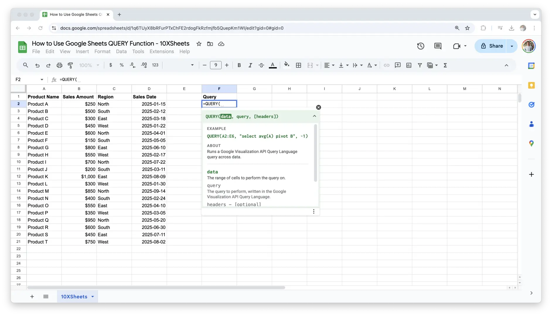
Google Sheets QUERY Function Syntax

The syntax for Google Sheets QUERY is straightforward and flexible. At its core, it follows this structure:

=QUERY(data, query, [headers])

• data: The range of cells you want to apply the query to (e.g., A1:B10).
• query: The actual query you want to run, written as a string of text. It defines the selection, filtering, sorting, and other operations.
• headers: This optional argument specifies how many rows in your data range are header rows. Typically, this is set to 1 if you have one header row, but it can be adjusted based on your data.

How to Write a Google Sheets QUERY?

Writing a basic query starts with identifying the data you want to analyze and then specifying the conditions for that analysis. For example, if you have sales data in the range A1:B10, where column A contains product names and column B contains sales amounts, a simple query to select the sales data might look like this:

=QUERY(A1:B10, "SELECT B", 1)

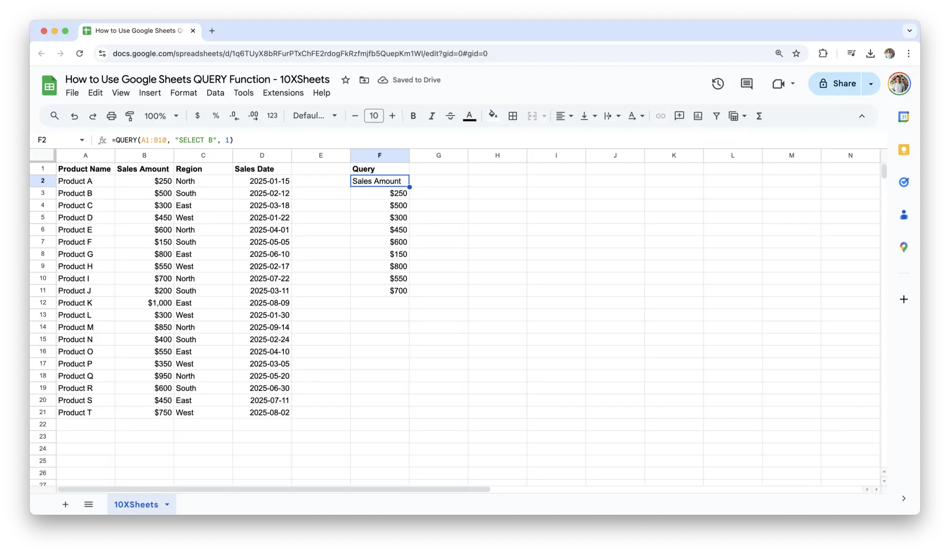
This query will return all the values in column B (sales), excluding column A (product names). It’s simple and gets straight to the point.

To make it more advanced, you could add a condition to filter the results. For instance, if you want to see only the sales amounts greater than $500, you could write:

=QUERY(A1:B10, "SELECT B WHERE B > 500", 1)

This will return only the sales values that are greater than $500, allowing you to focus on larger transactions.

Key Google Sheets QUERY Terms

• SELECT: Specifies the columns you want to retrieve from your data.
• WHERE: Defines conditions to filter the rows you want based on specific criteria.
• ORDER BY: Organizes the data in a specific order (ascending or descending).
• LIMIT: Restricts the number of rows returned by the query.
• GROUP BY: Groups data by specified columns for aggregation (e.g., SUM, COUNT).
• HAVING: Filters grouped data after applying GROUP BY.
• ASC: Stands for ascending order (default when sorting).
• DESC: Stands for descending order (used when sorting data from high to low).

How to Use Google Sheets QUERY Function?

Once you’re comfortable with the basics, it’s time to dive into advanced queries that offer more control over how you display and analyze your data. This section covers how to fine-tune your queries using the SELECT clause to choose specific columns, filter data with WHERE, sort results with ORDER BY, and limit the number of rows returned with LIMIT.

1. Use SELECT to Choose Specific Columns

When you work with data in Google Sheets, it’s rare that you need every column from a dataset. With the SELECT clause in the QUERY function, you can specify exactly which columns you want to pull from your data range. This gives you greater control and makes your results easier to read.

For example, let’s say you have a table with sales data, where column A is the product name, column B is the sales amount, and column C is the region. If you only need the sales amounts (column B), you can write a query like this:

=QUERY(A1:C10, "SELECT B", 1)

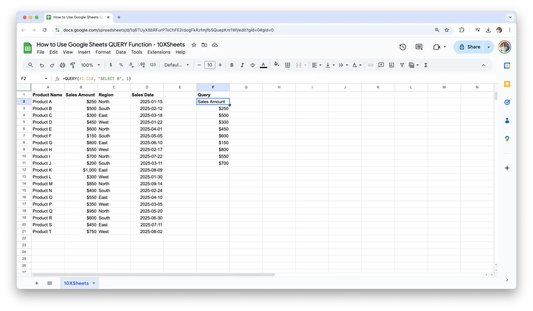
This query will return only the data in column B (sales amount), ignoring other columns in the range. If you wanted to pull both product names and sales amounts, you could adjust your query like so:

=QUERY(A1:C10, "SELECT A, B", 1)

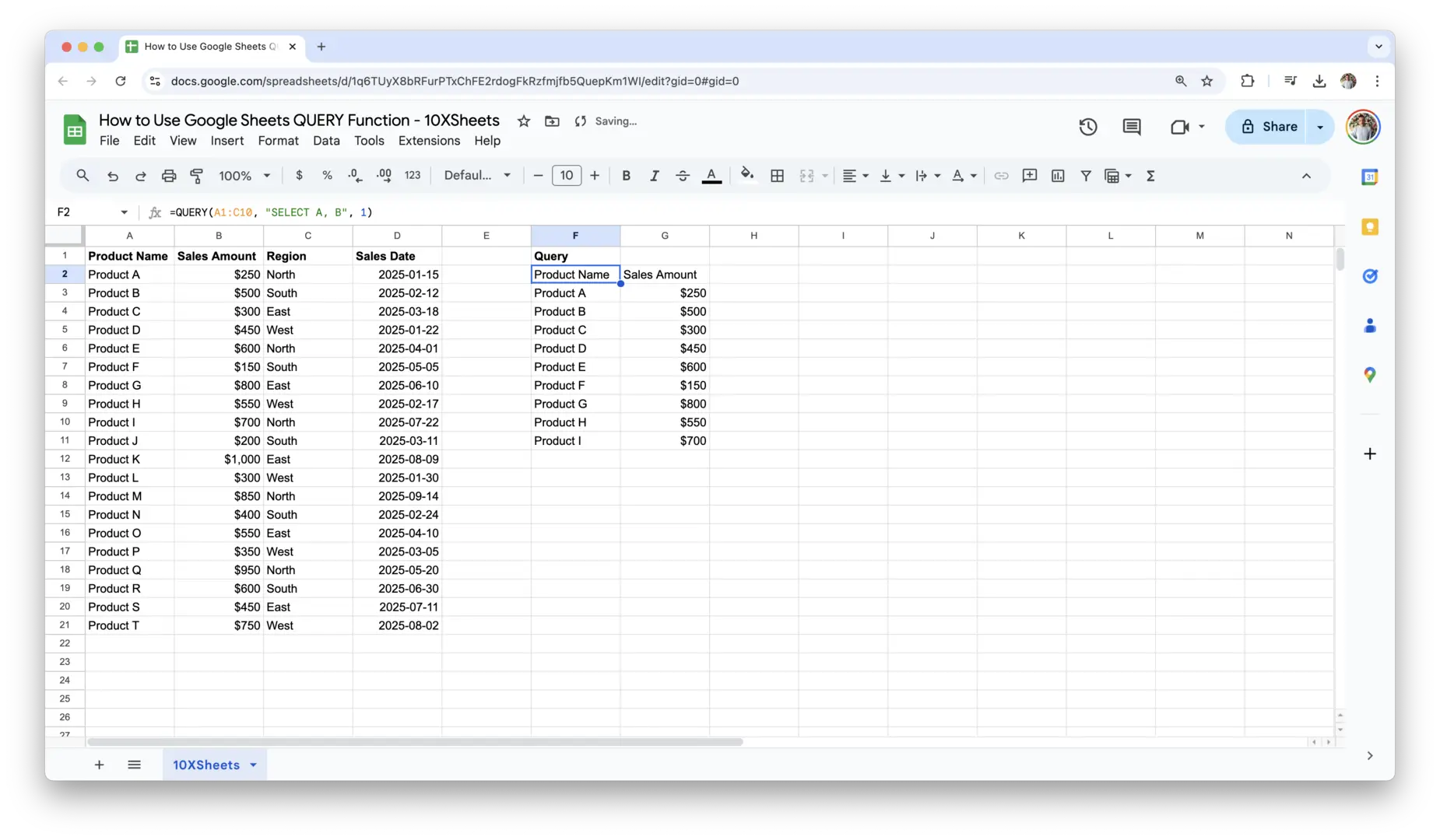
By specifying columns explicitly, you can avoid cluttering your results with irrelevant data. The SELECT clause can also include more complex expressions, such as calculated fields. For example, if you wanted to display the total sales in column B multiplied by a fixed amount of 2, you could write:

=QUERY(A1:D10, "SELECT A, B, B * 2", 1)

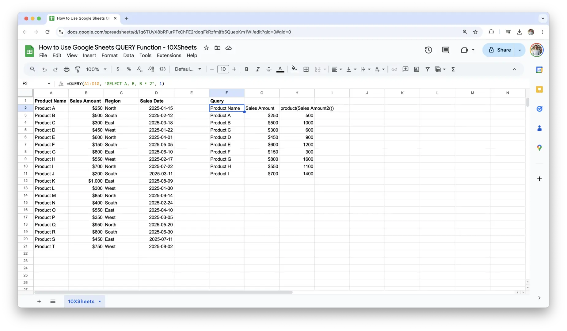
This provides much-needed flexibility when you’re analyzing specific columns or performing custom calculations.

2. Filter Data with WHERE

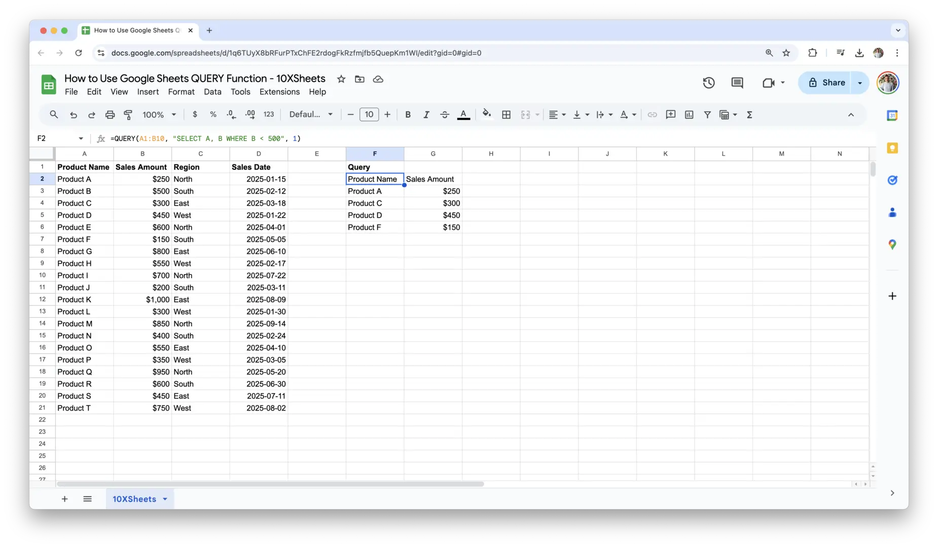
The WHERE clause is essential when you need to filter data based on certain criteria. It allows you to narrow down your dataset to only the rows that meet the conditions you specify. For example, if you want to pull sales data for only products that had sales greater than $500, you could write:

=QUERY(A1:B10, "SELECT A, B WHERE B > 500", 1)

This query will return the product names (column A) and sales (column B) for rows where the sales amount is greater than 500. The WHERE clause can handle a wide range of conditions, including text, numeric comparisons, and even dates.

You can also combine multiple conditions using logical operators like AND, OR, and NOT. For instance, if you want to see products with sales greater than 500 but less than 800, use this query:

=QUERY(A1:B10, "SELECT A, B WHERE B > 500 AND B < 800", 1)

This query will only return the products with sales figures in that specific range. Similarly, you can filter text data by using conditions like WHERE A = 'Product X' or exclude certain values using NOT.

3. Sort Data with ORDER BY

Once you’ve selected and filtered the data you want, it’s often helpful to organize it. The ORDER BY clause allows you to sort your results based on one or more columns. Sorting can be done in either ascending or descending order.

For example, if you want to display your product names alongside their sales, sorted by sales in descending order, you can use this query:

=QUERY(A1:B10, "SELECT A, B ORDER BY B DESC", 1)

This will return a list of products and their sales amounts, sorted from the highest to the lowest sales.

You can also sort by multiple columns. For example, if you wanted to sort by sales in descending order first, and then by product name in ascending order, you can write:

=QUERY(A1:B10, "SELECT A, B ORDER BY B DESC, A ASC", 1)

This will first sort by the sales amount and then, for products with the same sales value, it will sort by product name alphabetically. Sorting is incredibly useful for organizing large datasets and ensuring you’re focusing on the most relevant data.

4. Limit Data with LIMIT

There are times when you only need to work with a small portion of your data, such as when you want to analyze just the top 10 best-selling products. The LIMIT clause helps you do exactly that by restricting the number of rows that your query returns.

For example, if you only wanted to display the first 5 rows of your sales data, sorted by the highest sales, you could write:

=QUERY(A1:B10, "SELECT A, B ORDER BY B DESC LIMIT 5", 1)

This query will return the top 5 products with the highest sales, sorted in descending order. By using the LIMIT clause, you can focus on the most important results without overwhelming yourself with too much data.

LIMIT is especially useful when you have large datasets and need to break them down into more manageable parts. For example, you could use LIMIT in combination with sorting to get the top 10 products in sales, then apply the same logic to get the bottom 10, or other slices of your data.

Each of these advanced techniques—SELECT, WHERE, ORDER BY, and LIMIT—enables you to create more customized, focused results in Google Sheets. Mastering these commands will allow you to manipulate your data more effectively, helping you make informed decisions faster and with greater accuracy.

Working with Google Sheets Operators and Functions

When working with the Google Sheets QUERY function, operators and functions are your tools for refining your results and performing advanced calculations. These elements give you the flexibility to tailor your queries exactly to your needs. Whether you’re looking to combine multiple conditions, compare values, manipulate text, or work with dates, understanding how to use operators and functions effectively will make you a power user of Google Sheets.

Logical Operators

Logical operators are essential when you need to combine multiple conditions in a query. They allow you to filter your data based on more than one criterion. The primary logical operators in Google Sheets QUERY are AND, OR, and NOT. These operators help you specify more complex conditions and extract data that meets multiple criteria.

For example, if you want to return products where the sales are greater than $500 and the region is “North”, you can use the AND operator like this:

=QUERY(A1:C10, "SELECT A, B WHERE B > 500 AND C = 'North'", 1)

This query will return the product names (column A) and sales (column B) for rows where the sales amount is greater than $500 and the region in column C is “North”. Both conditions must be true for the row to appear in the result.

You can also use OR when you want to filter data that meets at least one of several conditions. For instance, to return products where the sales are either greater than $500 or the region is “South”, you would write:

=QUERY(A1:C10, "SELECT A, B WHERE B > 500 OR C = 'South'", 1)

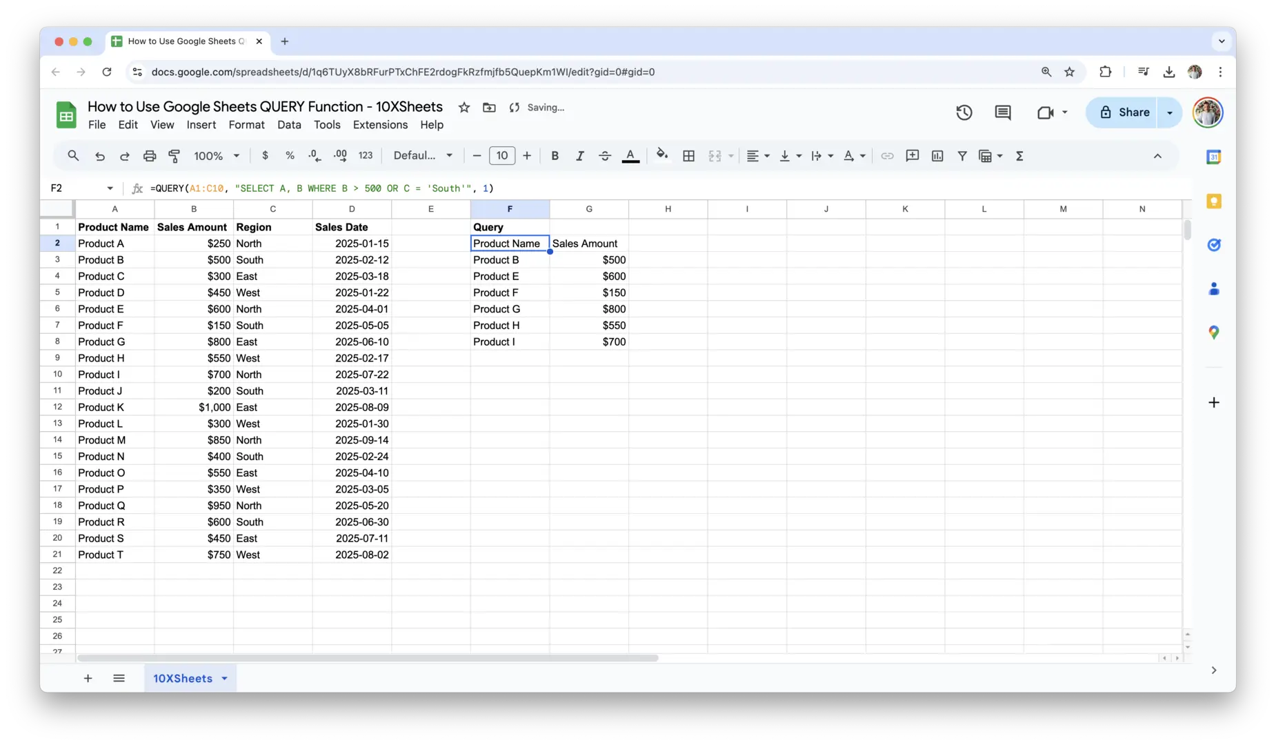
This query will return the product names and sales values for rows where either the sales amount is over $500 or the region is “South”. Using OR is helpful when you want to broaden your search criteria.

Lastly, the NOT operator lets you exclude certain data. For example, to exclude any rows where the region is “South”, you could write:

=QUERY(A1:C10, "SELECT A, B WHERE NOT C = 'South'", 1)

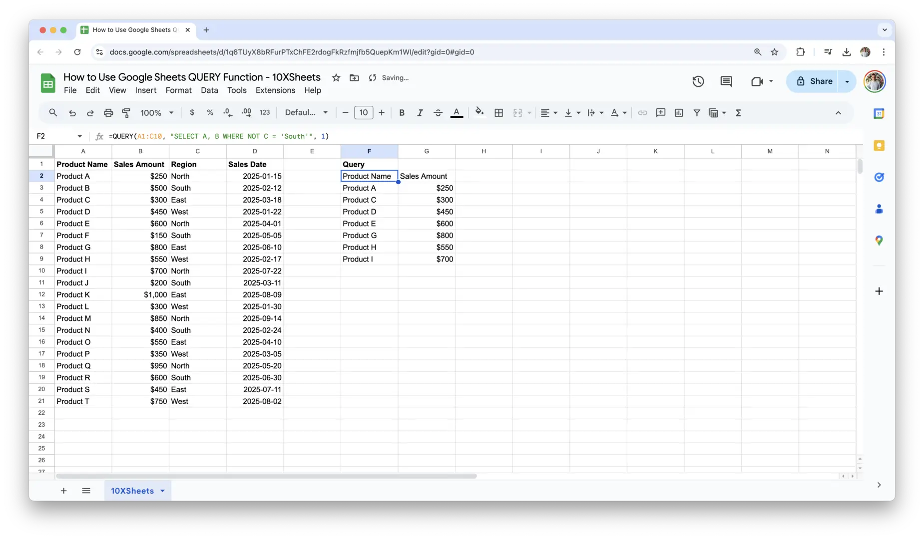
This will return all products and sales where the region is not “South”.

Comparison Operators

Comparison operators allow you to compare values in your data and filter your query results accordingly. These operators are essential when you’re looking for specific data points or ranges. The most common comparison operators are =, >, <, >=, <=, and <> (not equal to).

If you want to filter products based on sales greater than $500, use the greater-than operator (>):

=QUERY(A1:B10, "SELECT A, B WHERE B > 500", 1)

This query will return all product names (column A) and their sales amounts (column B) where the sales value is greater than $500.

You can also use the less-than operator (<). For example, if you want to find products with sales less than $500, write:

=QUERY(A1:B10, "SELECT A, B WHERE B < 500", 1)

This will return the products with sales lower than $100.

To check for values that are equal to a specific number, use the equals operator (=). For example, to get all products with sales exactly equal to $250, write:

=QUERY(A1:B10, "SELECT A, B WHERE B = 250", 1)

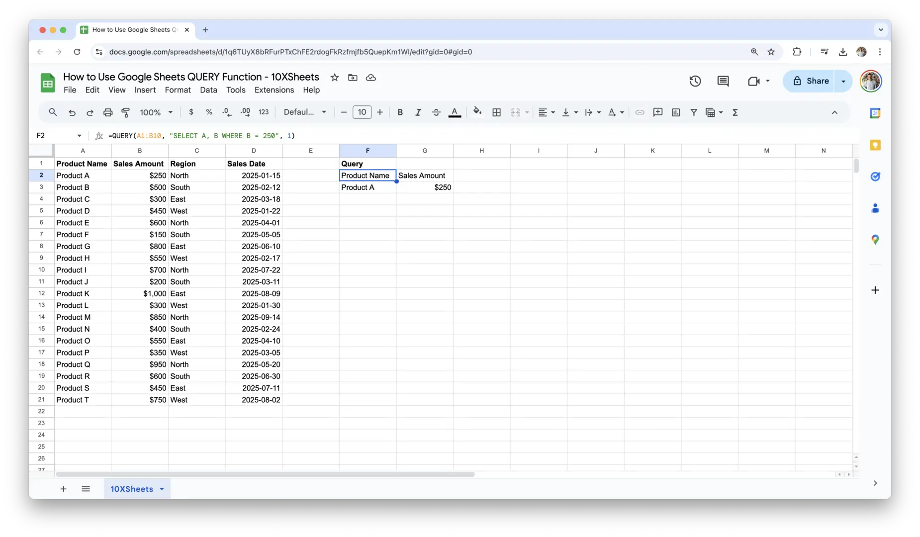
This will return only the rows where sales are exactly $200.

You can also use the greater-than-or-equal (>=) and less-than-or-equal (<=) operators when you want to include data that meets or exceeds certain values. For example:

=QUERY(A1:B10, "SELECT A, B WHERE B >= 500", 1)

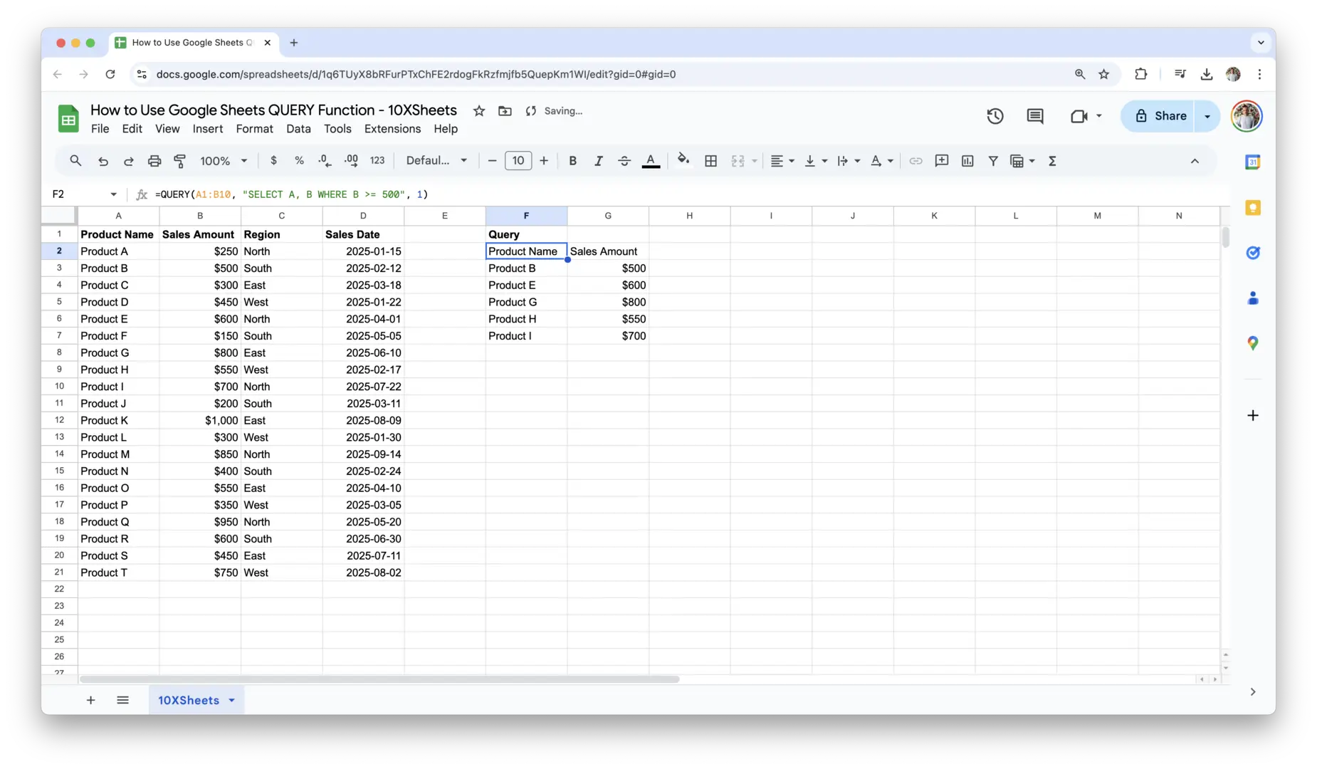
This will return all rows where sales are greater than or equal to $500.

If you need to exclude specific values, use the <> (not equal to) operator. For example, to exclude products with sales of exactly $300:

=QUERY(A1:B10, "SELECT A, B WHERE B <> 300", 1)

This will return all products except those with sales of $300.

Text Functions

Text functions allow you to manipulate or analyze text data within your queries. These functions are especially useful when you need to standardize or transform text values before displaying them in your results. Some of the most commonly used text functions in Google Sheets QUERY are CONCATENATE, LOWER, and UPPER.

For example, if you want to display all product names in lowercase, you can use the LOWER function. This is helpful when you want to ensure consistency, particularly if your data includes mixed-case entries:

=QUERY(A1:B10, "SELECT LOWER(A), B", 1)

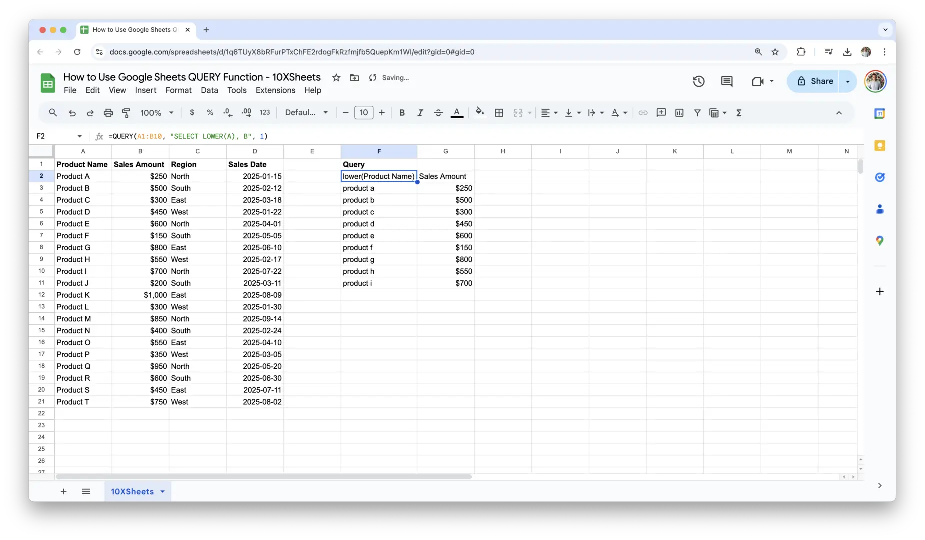
This query will return the product names in lowercase, along with their sales figures.

Similarly, the UPPER function converts text to uppercase. If you want to display product names in uppercase, you can write:

=QUERY(A1:B10, "SELECT UPPER(A), B", 1)

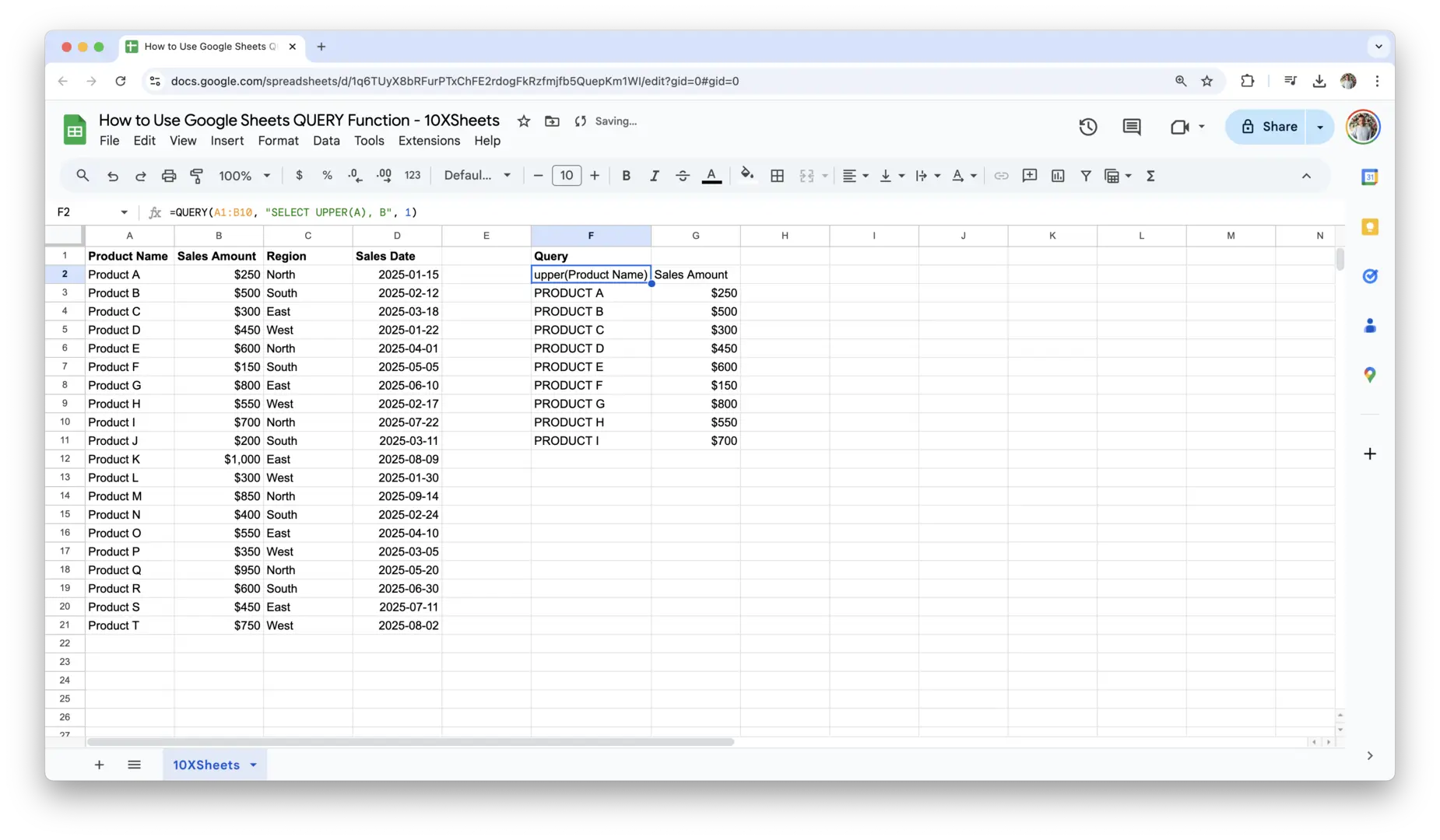
This will return product names in all caps, making them stand out more in your results.

The CONCATENATE function allows you to combine multiple columns into a single one. For example, if you want to merge the product name and the sales amount into a single column, you could use:

=QUERY(A1:B10, "SELECT CONCATENATE(A, ' - ', B)", 1)

This will display the product name followed by its sales amount in one column, separated by a dash.

These text functions help you customize how your text data appears and streamline your analysis when you need to transform values before reporting them.

Date Functions

Google Sheets QUERY also supports various date functions that allow you to work with dates effectively. Date functions like YEAR, MONTH, and DAY let you extract parts of a date for further analysis.

For example, if you have a column with dates and want to extract just the year from each date, you can use the YEAR function:

=QUERY(A1:D10, "SELECT YEAR(D)", 1)

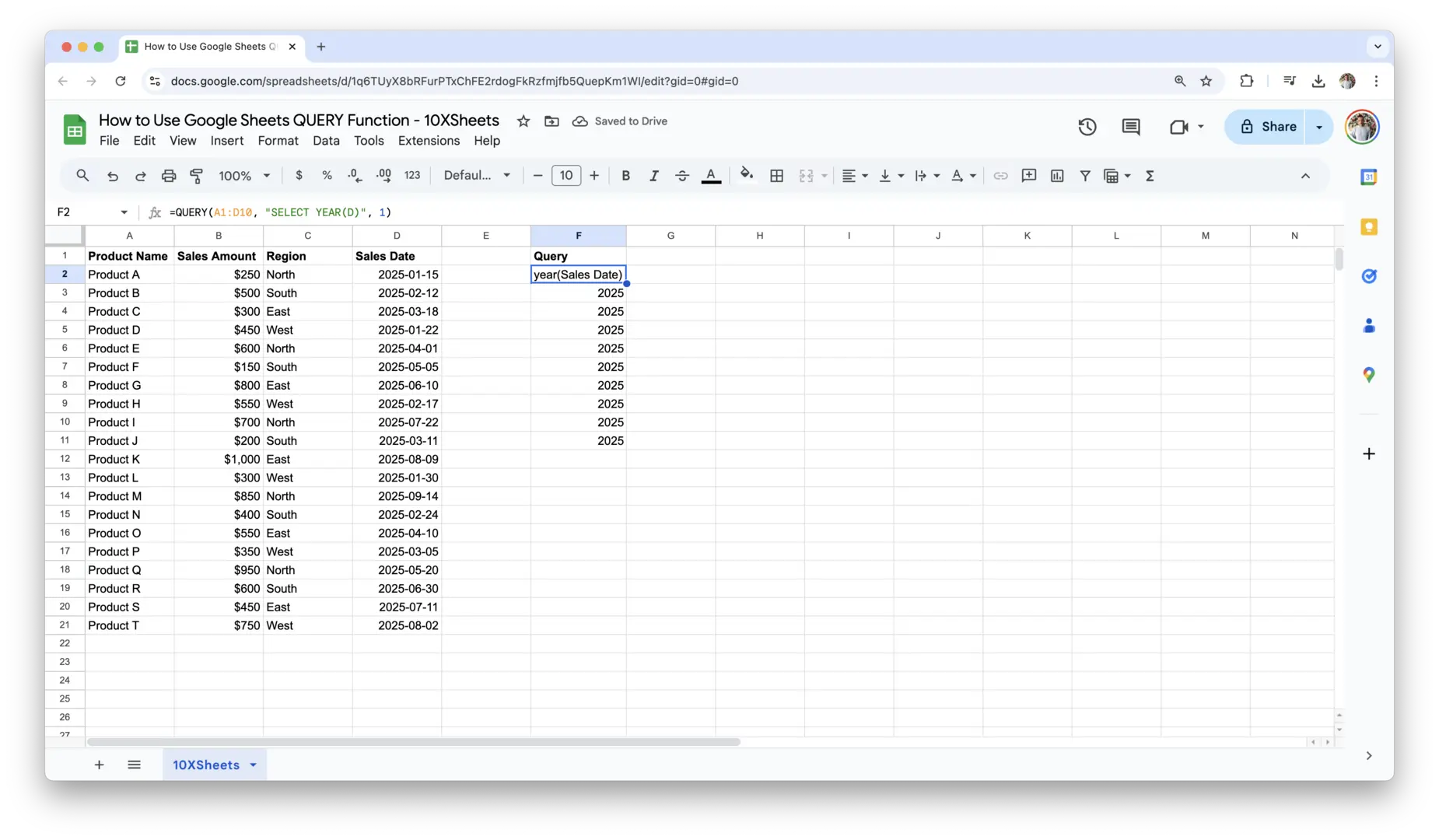
This query will return the year from the dates in column C, allowing you to analyze your data by year rather than by full date.

Similarly, you can use the MONTH function to pull the month from a date. If you want to display the sales data for each month, use:

=QUERY(A1:D10, "SELECT MONTH(D), SUM(B) GROUP BY MONTH(D)", 1)

This will return the total sales for each month, assuming that column C contains the dates and column B contains the sales data.

If you need to extract the day of the month, use the DAY function. For instance:

=QUERY(A1:D10, "SELECT DAY(D), SUM(B) GROUP BY DAY(D)", 1)

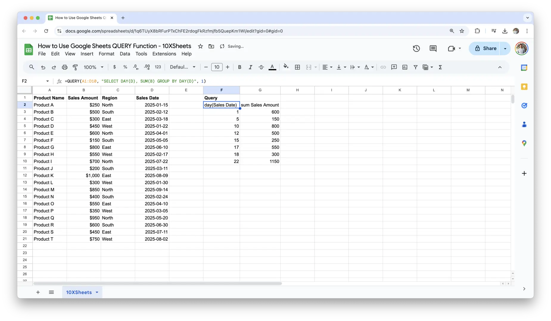
This query will return the total sales for each day of the month, assuming column C contains the dates and column B contains the sales values.

Using these date functions, you can easily analyze trends over time, group data by year, month, or day, and make time-based comparisons within your dataset. Date functions are powerful tools for anyone working with time-sensitive data in Google Sheets.

By mastering these operators and functions, you can turn simple queries into sophisticated data analysis tools. They allow you to customize and filter your results in ways that fit your exact needs, from comparing sales figures to transforming text data or extracting specific date information.

How to Combine Data with Multiple Tables?

In real-world scenarios, you often need to analyze data from multiple sources or tables in one query. Fortunately, Google Sheets QUERY function allows you to combine data from different ranges, sheets, or even use advanced formulas to bring everything together. Let’s explore how you can manage multiple tables and datasets efficiently.

Using Multiple Ranges in a QUERY

When you have multiple data ranges in the same sheet, you can combine them in a single query using curly braces {}. This is particularly useful when you have data scattered across different sections of the sheet, but you want to analyze them together.

For example, if you have sales data in A1:B10 and another set of data in A11:B20, you can combine both ranges in one query like this:

=QUERY({A1:B10; A11:B20}, "SELECT A, B", 1)

The curly braces {} allow you to combine the two ranges into one unified data set. The semicolon ; is used to stack the ranges vertically, while a comma , would be used to combine ranges horizontally. This approach is useful when you want to analyze data from different sections of a sheet without manually copying and pasting the data into one continuous range.

Joining Data from Different Sheets

If your data is spread across different sheets within the same workbook, Google Sheets QUERY lets you reference other sheets directly in your query. This makes it easy to pull in related data and join it for analysis, even if the data isn’t in the same table.

Let’s say you have sales data in sheets 10XSheets and data in Sheet 2. To combine both datasets in one query, you could use:

=QUERY({'10XSheets'!A1:B10; 'Sheet 2'!A11:B21}, "SELECT Col1, Col2", 0)

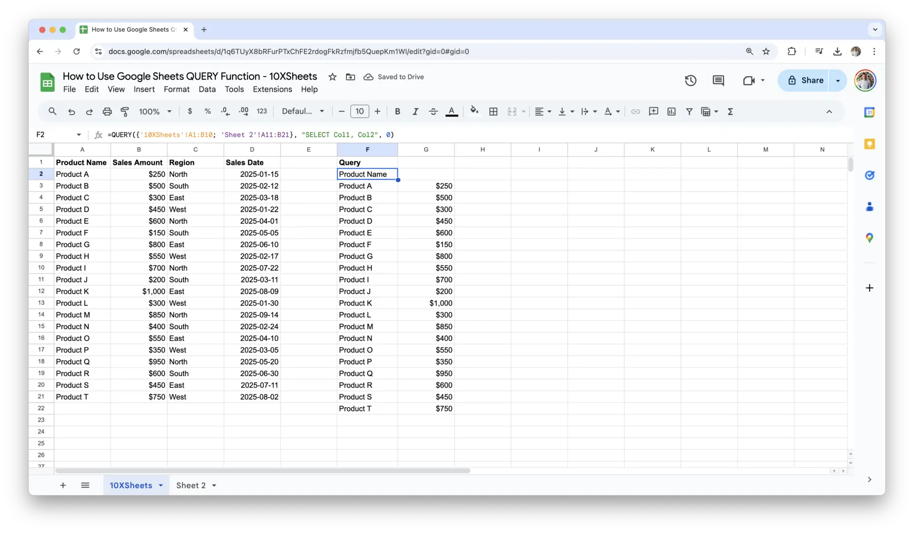
In this case, {Sheet1!A1:B10; Sheet2!A1:B10} combines data from both sheets into a single range, and the query selects the first two columns from each dataset. You can modify the query to filter, sort, or analyze the data just like you would for data in a single sheet.

If you want to join data from two sheets and match rows based on a shared key (for example, a product ID), you’ll need to get creative. While Google Sheets QUERY doesn’t support full SQL-style JOINs, you can mimic this behavior by ensuring both datasets are aligned and using array formulas or auxiliary columns.

Using Array Formulas and QUERY Together

Array formulas in Google Sheets are incredibly powerful when combined with the QUERY function. An array formula allows you to apply a formula to a range of cells, and you can use this to manipulate your data before passing it through a query.

For example, suppose you have a list of sales values in column B and you want to increase each sale by 10% before running a query. You could use the ARRAYFORMULA function combined with QUERY to automatically adjust the sales data:

=QUERY(ARRAYFORMULA(B1:B10 * 1.1), "SELECT Col1", 1)

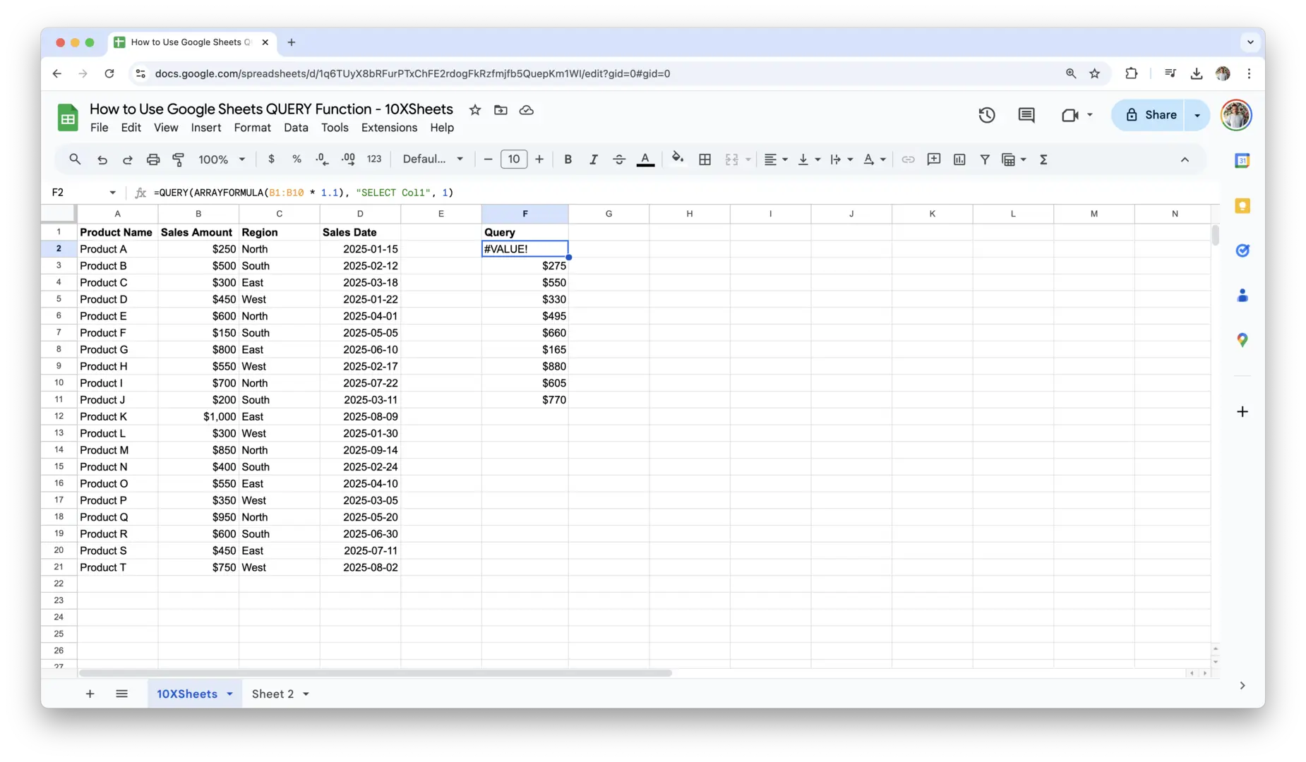
In this query, ARRAYFORMULA(B1:B10 * 1.1) multiplies each value in the range B1:B10 by 1.1 (increasing the sales by 10%), and then the QUERY function returns the adjusted values. Array formulas help when you need to preprocess data before querying it, and they can handle a wide range of calculations or transformations.

Combining arrays and queries allows for more dynamic and complex analyses, such as conditional calculations, transformations, and aggregations that would otherwise require multiple steps.

Google Sheets QUERY Examples and Use Cases

Using Google Sheets QUERY in the real world can transform how you handle data analysis, making complex tasks quick and easy. Below are a few examples that show how you can apply these techniques to common scenarios.

Summarizing Sales Data by Region

Let’s say you have a table of sales data where column A contains product names, column B contains sales amounts, and column C contains the region in which each product was sold. If you want to summarize the total sales by region, you can use Google Sheets QUERY to aggregate the data.

Here’s how you might write a query to calculate the total sales per region:

=QUERY(A1:C10, "SELECT C, SUM(B) GROUP BY C", 1)

This query groups the sales data by the region (column C) and sums up the sales amounts (column B) for each region. It’s a quick way to generate a summary of sales by region without needing to manually filter and calculate totals.

If you want to see the results sorted from the highest to the lowest sales, you can add an ORDER BY clause:

=QUERY(A1:C10, "SELECT C, SUM(B) GROUP BY C ORDER BY SUM(B) DESC", 1)

This will show the regions with the highest total sales at the top, making it easier to compare the performance of different regions at a glance.

Filtering Employees Based on Criteria

Imagine you have a list of employees, with columns that include name, department, and salary. You can use a query to filter employees based on specific criteria, such as filtering for employees in a particular department with a salary above a certain threshold.

For example, to filter employees in the “Sales” department who earn more than $50,000, you could write:

=QUERY(A1:C10, "SELECT A, B, C WHERE B = 'Sales' AND C > 50000", 1)

This query will return the names (column A), departments (column B), and salaries (column C) for all employees who meet the criteria. The WHERE clause ensures that only employees in the Sales department with salaries above $50,000 are included in the result.

Queries like this are incredibly helpful for HR departments or any situation where you need to filter large amounts of data based on multiple conditions. You can apply different filters, such as selecting employees by job title, performance rating, or tenure, depending on your needs.

Sorting and Limiting QUERY Results

When working with large datasets, you might only need to focus on the top or bottom results. You can use the ORDER BY clause to sort the data and the LIMIT clause to restrict the number of results.

For example, suppose you have a list of products with their sales amounts, and you only want to display the top 5 best-selling products. You could write:

=QUERY(A1:B10, "SELECT A, B ORDER BY B DESC LIMIT 5", 1)

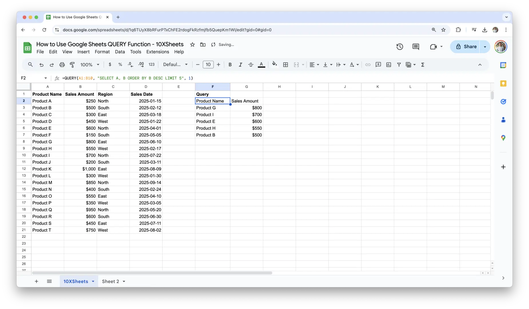
This query will return the top 5 products based on the highest sales figures, sorted in descending order.

Similarly, if you wanted to focus on the bottom 5 products in terms of sales, you can change the ORDER BY clause to ASC for ascending order:

=QUERY(A1:B10, "SELECT A, B ORDER BY B ASC LIMIT 5", 1)

Sorting and limiting results help you quickly identify trends, such as top performers or underperformers, and make it easier to focus on the data that matters most.

These examples demonstrate just a few of the countless ways you can use Google Sheets QUERY to streamline your data analysis. Whether you’re summarizing, filtering, sorting, or limiting data, Query functions let you customize how you interact with your data and make it easier to draw meaningful insights quickly.

Best Practices for Using Google Sheets QUERY

To make the most out of the Google Sheets QUERY function, following a few best practices can enhance your productivity, ensure your queries are optimized, and help you manage your data more effectively. These tips will guide you toward using the QUERY function more efficiently and avoid common pitfalls.

• Keep your data organized: Structure your data with clear headers, ensure consistency in column formats, and avoid mixing data types (e.g., text with numbers) within the same column.
• Use named ranges for clarity: Instead of referencing cell ranges like A1:B1000, create named ranges to make your queries easier to read and manage.
• Avoid complex queries on large datasets: For faster performance, break up large queries into smaller, more manageable parts. Consider using filters and smaller data ranges to speed up the execution.
• Leverage array formulas for preprocessing: Use ARRAYFORMULA to perform calculations or transformations on data before querying, which can make your queries more dynamic.
• Limit the use of volatile functions: Functions like NOW() or RAND() can slow down your queries, so use them sparingly, especially in large datasets.
• Use helper columns when necessary: If you need to perform complex calculations or transformations, create additional columns in your data to help structure the query results.
• Test your queries step-by-step: If your query isn’t returning the expected results, start with a simple query and build it incrementally, adding one condition or function at a time.
• Opt for clear and specific conditions in WHERE clauses: Always make your filtering conditions clear and as specific as possible to avoid returning unnecessary data.
• Keep an eye on data updates: When your data changes frequently, make sure your queries are set up to dynamically update or recalculate as needed, keeping your analysis up-to-date.

Handling Google Sheets QUERY Errors and Troubleshooting

Even the most seasoned Google Sheets users can encounter errors when writing complex queries. Knowing how to troubleshoot and resolve common issues will save you time and frustration. Below are some tips for handling and fixing errors in your queries.

• Check your query syntax: Syntax errors are common, especially with quotation marks, commas, or missing parentheses. Double-check for these errors, particularly in the query string.
• Ensure column references are correct: Ensure that you are referencing the correct columns in your SELECT and WHERE clauses. If you use {} to combine multiple ranges, make sure your column references match across all ranges.
• Confirm the correct number of header rows: If your data range includes multiple header rows, adjust the header parameter in your query to match the number of rows containing headers. The default is usually 1.
• Look for incorrect data types: If you’re comparing text and numbers, or dates in the wrong format, your query might not return results as expected. Ensure data consistency within columns.
• Use ISBLANK for missing data: If you’re getting unexpected results due to blank cells, use the ISBLANK function in your query to handle or exclude blank values in your dataset.
• Recalculate and refresh your sheet: Sometimes errors can be caused by outdated data or stale calculations. Refresh your sheet or re-enter your query to ensure everything is up-to-date.
• Be mindful of the data range: Ensure that your query is referring to the correct range and that the range is large enough to include all necessary data.
• Check for non-visible characters: In some cases, non-visible characters like spaces or line breaks can cause issues with comparisons in the WHERE clause. Use the TRIM() function if necessary to clean up your data.
• Break down complex queries: If your query is not working as expected, break it down into simpler parts and check each step individually to isolate the problem. You can also try writing a simpler query to verify the dataset itself is correct.

Conclusion

Now that you’ve learned the basics and advanced techniques of Google Sheets QUERY, you have a powerful tool at your fingertips to analyze and manage data more efficiently. Whether you’re filtering large datasets, summarizing information, or joining data from multiple sheets, QUERY allows you to do all of this with just a few simple formulas. The flexibility and simplicity of this tool make it perfect for anyone looking to streamline their data analysis, from beginners to advanced users.

Remember, the more you practice with Google Sheets QUERY, the more comfortable you’ll become with writing complex queries and customizing them to fit your specific needs. Keep experimenting with different functions and features like sorting, grouping, and combining data from multiple sources. The more you use it, the more you’ll discover how much time and effort QUERY can save you, making data analysis smoother and quicker. By mastering this tool, you’ll be able to handle even the most complicated datasets with ease.